A VAE differs from a plain autoencoder in one non-negotiable way. The encoder does not output one latent vector. It outputs parameters of a distribution, then training samples from that distribution and decodes the sample. That small change is why a VAE can generate new examples by sampling from a known latent space instead of only reconstructing inputs.
Scope: build intuition for the moving parts, then connect them to failure symptoms you can observe on real runs.
The encoder outputs uncertainty on purpose
A plain autoencoder learns a function that maps an input to a single code , then another function that maps back to a reconstruction . If you try to generate, you pick a random and decode it. The decoder usually outputs garbage because the encoder only ever produced codes on a thin, irregular surface inside latent space.
A VAE avoids that by having the encoder output two vectors for each input. One vector controls where the code tends to land, and one controls how spread out it is. Concretely, the encoder outputs a mean and a standard deviation , which define a Gaussian distribution . Training samples from that distribution, then decodes .
That means the same input can yield slightly different samples and slightly different reconstructions. The goal is not randomness for its own sake. The goal is to make nearby latent points decode to similar outputs, so generation becomes predictable.
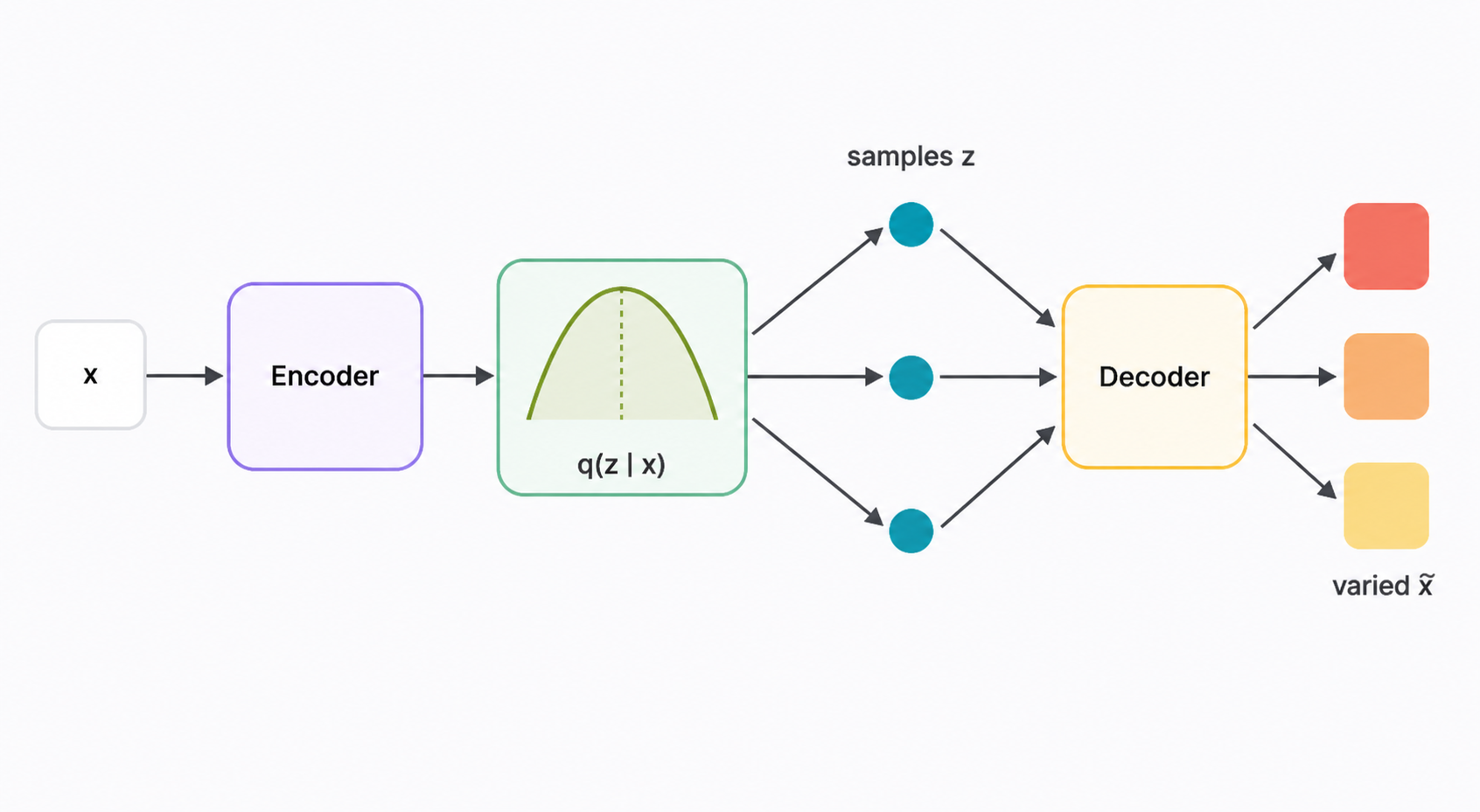
Once the encoder outputs a distribution, training needs a reason to keep those distributions well-behaved across the dataset. That is where the loss changes.
From autoencoder to VAE loss
A VAE trains with two competing pressures. One pressure says reconstruct the input accurately. The other says do not let the per-input latent distribution drift too far from a simple reference distribution, typically a standard normal .
A common objective is the negative evidence lower bound, which appears in code as reconstruction loss plus a KL term.
Here is the encoder distribution, is the decoder likelihood, and is the reference prior, often . The first term punishes reconstructions that miss details. The second term punishes encodings whose mean drifts far from or whose variance becomes extreme, because both make sampling from unlikely to land in regions the decoder has seen.
Rule of thumb: If samples from random look bad, the latent space is probably not aligned with the prior, and the KL term is too weak, too late, or being ignored in practice.
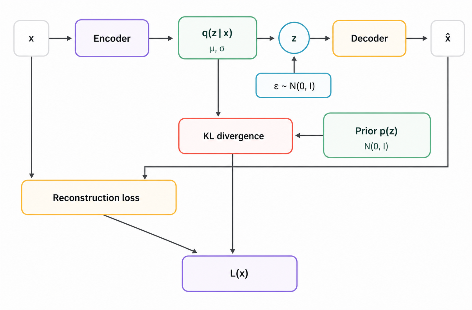
With the loss in place, it helps to see what data actually moves through the network during a forward pass.
What happens in a VAE forward pass
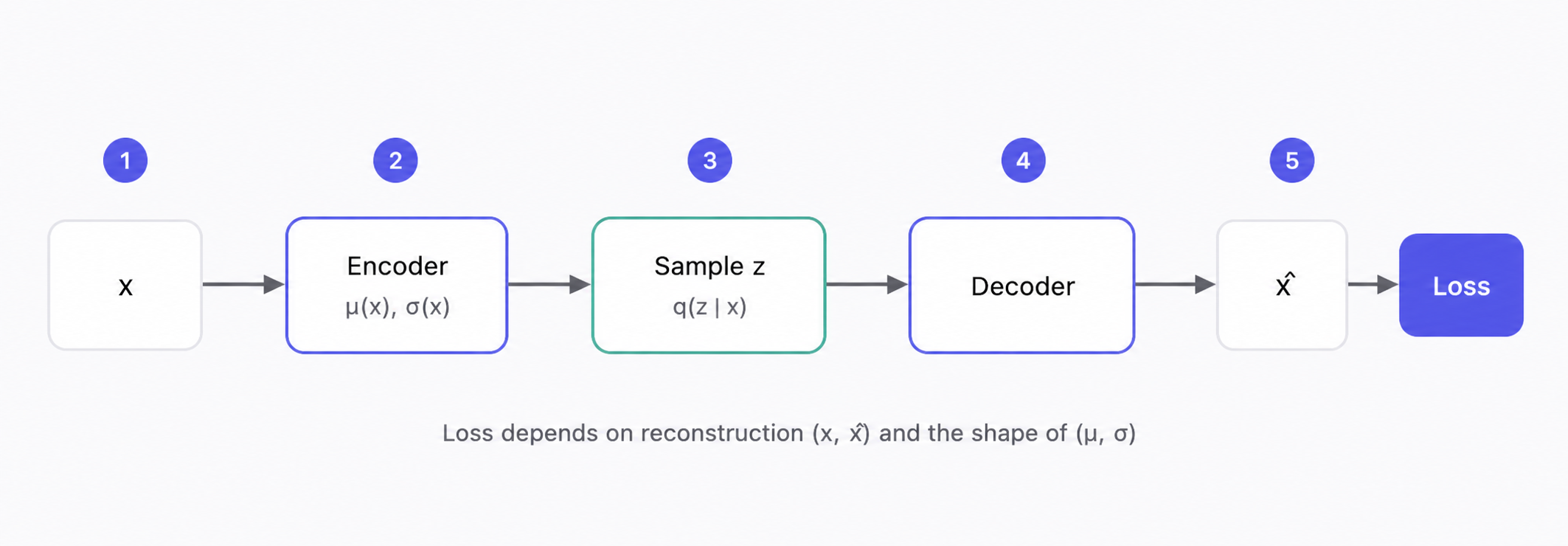
A VAE forward pass is a short pipeline that alternates between deterministic computation and one stochastic step.
Step-by-step behavior
- Start with an input .
- The encoder outputs and .
- A latent sample is drawn from using those parameters.
- The decoder maps to a reconstruction .
- The training loop computes reconstruction loss from and KL divergence from .
The important practical point is that the loss depends on both the reconstruction and the shape of the encoder distribution. A VAE can show low reconstruction error while still failing at generation if the KL term is not shaping latent space.
Sampling looks like it blocks backpropagation because sampling is not a smooth function of network weights. Training works anyway because the sampling step is rewritten as a differentiable computation.
Reparameterization trick and why it matters
Backpropagation needs a gradient that tells each weight how to change to reduce loss. If were sampled directly from , the graph would include a random draw that does not provide a usable gradient path back to and .
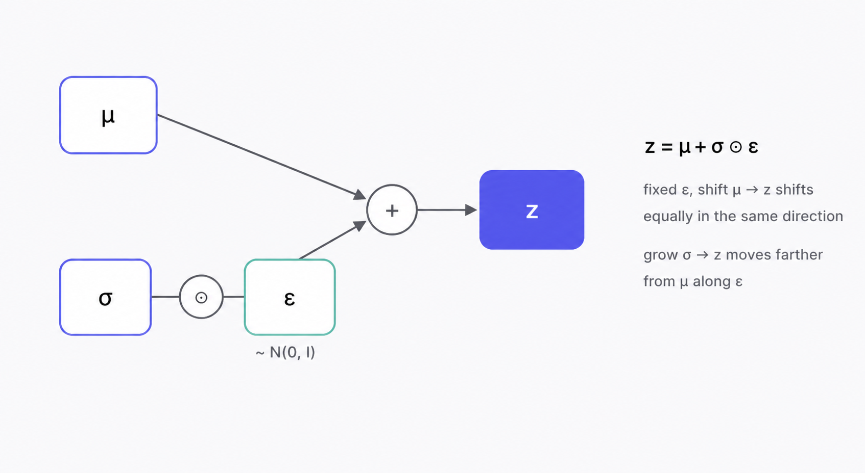
The workaround is to sample noise that is independent of the encoder output, then transform it.
is standard normal noise, and is elementwise multiplication. Now is a deterministic function of for a fixed sample, so gradients can flow into and through ordinary differentiable operations.
A concrete way to sanity check this is to hold fixed. If shifts, shifts by the same amount. If grows, moves farther from in the direction set by .
With reparameterization, the VAE can actually train. The next question is why the KL term is worth the reconstruction tradeoff you often see as blur.
What the KL term buys you in practice
A VAE works best when two behaviors hold at the same time. First, neighboring latent points decode to similar outputs. Second, points drawn from land in regions the decoder has been trained on. The KL term is the main reason both behaviors can happen together.
Without KL, the encoder can pack inputs into disconnected pockets anywhere in latent space, as long as the decoder can invert them. That makes interpolation and random sampling unreliable. With KL, each input distribution is pressured toward a shared, simple shape, which encourages continuity.
This does not guarantee perfect generation. It shifts failure modes into ones you can reason about and measure.
Plain autoencoder vs VAE
| Aspect | Plain autoencoder | VAE |
|---|---|---|
| Random sampling | Poor | Good |
| Interpolation | Unreliable | Smooth |
| Downstream use | Sometimes useful | Often useful |
| Typical failure mode | Latent holes, odd samples | Blurrier reconstructions |
That comparison points to the real workplace pain. Nothing crashes. Outputs just look wrong, or metrics stall. The fastest way to debug is to map a symptom to one likely cause and one likely change.
Use cases and failure modes you can recognize
VAEs show up in representation learning, semi-supervised learning, anomaly detection via reconstruction error, and as building blocks inside larger generative systems. In day-to-day work, the issues are usually visible in a handful of recurring symptoms.
Common trap: Better reconstruction is not always better generation. If the KL term collapses toward zero early, samples can get worse while reconstructions look fine.
Blurry reconstructions often mean the decoder is too powerful; reduce decoder capacity so the latent code carries more detail. Posterior collapse usually improves with KL annealing or a smaller .
A practical way to keep this from becoming guesswork is to watch a few signals and use one simple decision rule.
How to tell it is a VAE problem
Start with three plots that are cheap to track and usually diagnostic.
- Reconstruction loss over steps, on train and validation.
- KL divergence over steps, ideally per latent dimension as well as summed.
- Sample quality checks at fixed intervals by decoding , not just reconstructions.
The key patterns:
- If reconstruction improves but KL quickly goes to near zero and stays there, the encoder is not using latent capacity. That is posterior collapse. It often shows up when the decoder is strong enough to ignore , especially with autoregressive decoders in text.
- If KL grows without bound or samples look unstable, the encoder distributions are drifting away from the prior. Random sampling then lands in regions the decoder did not see during training.
- If both losses look reasonable but outputs are consistently blurry, the model is trading detail for average likelihood. Pixel-wise losses tend to do this on multimodal data.
A simple decision rule that works in many teams is this. If decoding random looks much worse than reconstructing , prioritize fixing KL behavior before tuning the decoder. The gap is the signature of a latent space that is not aligned with the prior.